Abstract

An article in a previous edition of this Journal outlined the evolution of project management over three distinct Eras. Eras 1 & 2 encapsulate conventional project management thinking, while Era 3 describes a Project Production Management framework that views projects as temporary production systems and applies Operations Science to optimize project delivery.

In this article, we elaborate upon a number of conclusions that can be drawn from applying this Era 3 framework to the optimization and control of project execution. Era 2 conventional thinking does not provide an accurate or robust understanding of how a production system behaves. This is because Era 2 thinking ignores variability and inventory, and their impact on a given production system including the delivery of a project. Era 2 project management thinking therefore does not effectively expose hidden, but important, risks to the delivery of a project. This “gap” is a major contributor to project cost and schedule overruns and the associated claims.

In this article, we describe how Project Production Management provides the means for identifying and resolving these hidden risks.

Keywords: Temporary Production System; Production System Optimization; Project Production Control; Inventory; WIP; Variability

Introduction

In an earlier article in this Journal [1], Shenoy and Zabelle traced the evolution of project management thinking, proposing that three distinct Eras characterize three distinct themes driving the development of project management thought. Era 1 covers the period from the 1900s to the 1940s that was preoccupied with the productivity of labor in factory settings. Era 2 covers the periods from the 1940s to the 1990s which concerned itself with improving the predictability of capital project outcomes. Together, Eras 1 and 2 comprise what we term “conventional” project management thinking, as codified by the Project Management Institute in a reference work such as the Project Management Body of Knowledge [2]. Eras 1 and 2 are distinguished from a third emerging Era that views projects as temporary production systems and applying Operations Science to improve the profitability of project execution.

In this paper, we elaborate upon several conclusions that can be drawn from Era 3 thinking [1], and contrast it with conventional Era 2 project management thinking [2]. The main contribution of this work is to explain the power of the Project Production Management framework to optimize and control project execution activities. We call these distinct applications Production System Optimization and Project Production Control.

Contrasting Era 2 Conventional Thinking with Era 3

Conventional thinking, based on accepted Project Management practice [2], establishes that there exists a cost / time trade-off (now extended to scope / quality, cost and time trade-off). In simple terms, it means it will cost more to deliver faster or take longer to deliver at less cost (as depicted while moving along the curve in Figure 1), wherein the only way to reduce both cost and schedule is to reduce quality / scope.

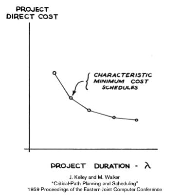
The technical basis for the trade-off shown in Figure 1 ignores variability and inventory, and their impact on a given production system. Conventional thinking does not provide an accurate or robust understanding of how a production system behaves, and therefore does not effectively expose these hidden, but important, risks.

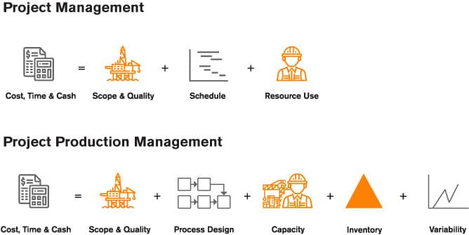
Figure 2 contrasts Era 2 conventional project management thinking with Era 3 “Project as Production System” thinking. The top row of Figure 2 shows the classical view of trading off scope / quality, schedule and resources to meet targets on cost and schedule. The bottom row of Figure 2 views a Project as a Production System, enabling explicit identification of risks typically hidden under a conventional project management perspective, including risks such as the presence of high variability and excessive inventory (work-in-process and stocks). Variability and inventory are not explicitly recognized in Era 2 conventional project management thinking, as suggested in Figure 2.

As explained in [3] [4], variability always degrades the performance of a production system. It cannot be completely eliminated but can be mitigated through process design. Residual variability must be buffered through a combination of inventory, capacity and time.

Understanding how variability, intentionally or unintentionally, results in excessive work-in-process (WIP) levels and capacity loss is important in order to understand the impact to project performance, including the ability to compress schedule and reduce cost, i.e., move the cost / time tradeoff curve, rather than just moving on the curve. This also opens new means to expose and identify risks that traditional thinking is blind to. Many projects continue to suffer the consequences of this blindness.

But, why are variability and WIP important in a situation where compressing schedule is imperative? Before we discuss variability, we will review a basic relationship that exists between Cycle Time (CT), Throughput (TH) and WIP, whether or not there is any variability. This relationship is known as Little’s Law [3], which states:

WIP is defined here as the total inventory between the start and endpoint of a process. As such, it can be located between individual operations (e.g., inventory of work to be done) or within an operation (work currently being done).

Since the TH rate is either the rate of releases or the rate of the bottleneck, whichever is less, WIP and CT are essentially a multiplicative constant of each other. In other words, WIP and CT are the same thing with different dimensions. Thus, we can say, “WIP is visible cycle time” and add that “WIP leads cycle time.” When you see WIP increase now, you will see CT (project duration) increase later.

There is a big problem if you try to control TH and push too much into the system: WIP and CT blow up. But the “blow up” is not immediate, it takes time. And, when the blow up occurs, it is too late to do anything about it, and thus all the attendant problems of cost overruns and schedule delays are now locked into the project. The future implications of WIP occur far in advance of being reported in project controls schedule updates and cost reports.

Of course, from a single trade perspective, the strategy of having plenty of WIP makes complete sense. As a matter of fact, it is very common for vendors and contractors to require large stocks to be placed before their operation in the form of information, materials and the completion of predecessor work. To this end, the application of methodologies such as Workface Planning and Advanced Work Packaging [5] are designed to ensure that these large inventory buffers are in place. Conventional construction measurements such as Productivity and Performance Factors (PF) can accentuate the increase in WIP.

Having massive amounts of WIP is useful for keeping contractors busy at high utilization rates. Contractors like this because they ostensibly can be more efficient and get paid sooner. But from the asset Owner Operator’s perspective, using measures such as Total Cost of Ownership (TCO,) this can be a terrible strategy. What invariably happens to projects with huge amounts of WIP is that contractors are busy, but they do not work in the correct sequence. They complete lots of work, but it is often not the work that was needed at the time and there is extensive interference between contractors. Large amounts of WIP means large amounts of effort associated with amassing, handling, holding, preserving and searching for WIP and, in many cases, large financial risk to the owner from WIP obsolescence due to engineering changes, deterioration due to weather, theft and other effects.

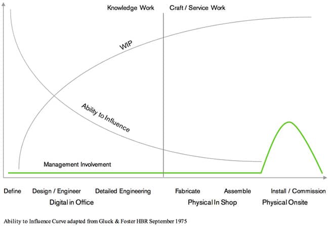
It gets worse on large projects that consist of many parallel operations where the use of WIP to shield work from variability is a very expensive recipe. Moreover, and as depicted in Figure 3 below, adapted from Gluck and Foster [6], experience from many projects usually indicates that WIP levels increase as a project moves through the delivery process. Additionally, management involvement usually comes too late and at that point there is little that they can do through conventional means to impact performance (e.g., reduce variability, control WIP levels, etc.).

Project Production Management

To understand how to reduce cycle time as the means to compress schedule, the components of cycle time must be clearly identified and well understood. Cycle time [3] has several components including Process Time (PT), Batch Time (BT), Set-up Time (ST), Move Time (MT) and Queue Time (QT), as per the following formula:

PT is the duration each unit of production that is worked within an operation. MT is the duration each unit of production spends being moved from one operation to another. ST is the duration each unit of production waits for an operation to be set up (such as increasing the height of a tower crane before working on upper floors). BT is the additional duration required to process a group of units treated as a batch rather than a single unit. BT is comprised of the following:

Though focus and efforts on reducing the process elements (PT+BT+MT+ST) of CT are quite common and better understood, a significant opportunity lies in understanding the impact of batch time (BT) and queue time (QT a.k.a., Wait Time) and how to reduce it.

Batch time can be reduced by working with smaller batches of work. This means that instead of working on a one-month group of tasks before moving on to the second group, work is divided into groups of two-day tasks. So, the third task can begin after four days instead of after two months. In other words, do more tasks in parallel when it is physically possible. Some will argue that it is less efficient to do this, that there is better productivity with one large crew doing one large task rather than several small crews doing smaller tasks. This may be true to some degree, but the improvement in terms of schedule and reduction of cash tied up in inventory commonly justify a slightly lower productivity.

The engineering and construction industry struggles to match the sequence of installation to the sequence provided by the supply. This is especially problematic when, for example, each pipe spool or steel member is unique. This mismatch of supply units with demand needs is called wait-to-match time. The result is more inventory and therefore more cycle time. This occurs whether the inventory is intentionally planned in an attempt to decouple supply and demand, or if no inventory is planned and yet the supply is not co-sequenced with the demand. The effect is the same – large amounts of inventory.

For example, suppose 7 sub-components are needed for each of 1000 unique pipe spools. Because the pipe spools are unique, each of the components could be unique. If the sequence of each component is randomly sequenced, the average “distance” between the first and the last will be 750 components.
If you are making 10 components per day, the average wait-in-batch time would by 7.5 days. And this inventory does not consider any randomness in the time to fabricate or the usage or the “stealing” of parts for use elsewhere or even backorder time. So, in practice, the amount of inventory caused by a lack of co-sequencing supply with demand is much larger.

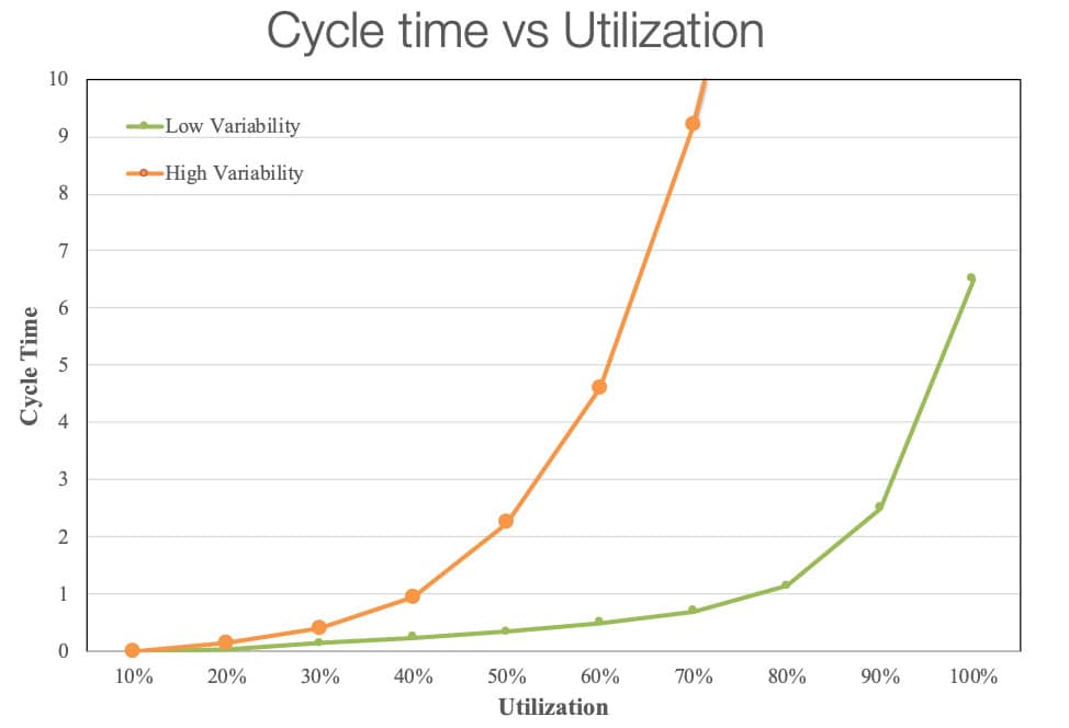
Often not considered in most scheduling systems and usually not even visible in project schedules, queue time (QT) is the aggregated amount of time that work remains between operations waiting to be executed (e.g., work waiting for capacity). The VUT equation below shows that the amount of QT is directly proportional to three multiplicative factors: (1) the amount of variability in both demand, c_a^2, and in the processes, c_e^2, (2) a non-linear capacity utilization factor, u/(1-u), and (3) the process time, PT. In practical terms, if we execute work within a given production system that is exposed to high levels of variability, QT will inevitably be higher, and therefore increase the overall cycle time.

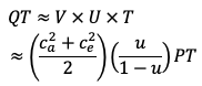
If we let the capacity utilization go to 100%, the QT will increase exponentially (refer to Figure 4 below). For instance, when capacity utilization levels of a highway system are high (meaning a lot of traffic), cars will inevitably stop, which means wait time increases. The key point is that the desire to reach 100% capacity utilization, especially in a highly variable environment, is counterproductive to the overall performance of a production system if the goal is to deliver the project within schedule and under budget, as illustrated in Figure 4.

Project Production Management considers all of these relationships. Key to its success is to deliver the project by (1) controlling WIP and (2) monitoring throughput daily. This results in a classic “pull” production system. While there is much confusion in the ‘Lean’ literature about push versus pull, the simple truth is that push occurs when one tries to control throughput and that pull is accomplished by using WIP as the control variable [7].

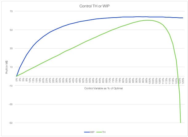
The key benefit of a pull system (i.e., controlling WIP rather than throughput) is that it is more robust to errors in execution [8]. While the push system is unforgiving when too much work is started, the pull system works well even with large errors in setting the WIP level. Figure 6 below shows this by comparing two models. Both models compute a net profit number from:

In other words, we get paid at a rate of p for each unit of throughput, but have a unit WIP expense representing the cost of capital and other WIP costs of c. We plot the performance of both systems in terms of their optimal control values, with 100% representing the optimal throughput or WIP. From the graph, we see there is a small difference between the two optimal values due to the tighter control of WIP versus throughput. But the more important difference is the fact that WIP performs well anywhere between 70% and 125% of optimal, whereas TH control drops off sharply just above the optimal value, yielding a negative net revenue at 123% of optimal.

Conclusion

In summary, the above Operations Science framework enables project teams to better understand, identify and expose risks that will be otherwise hidden with conventional practices, as well as influence Project Production System behavior. It is therefore essential to understand the unintended consequences of variability, high WIP levels and 100% capacity utilization targets.

References

1. R. G. Shenoy and T. R. Zabelle, “New Era Of Project Delivery – Project As Production System,” Journal of Project Production Management, vol. 1, no. Winter, 2016.

2. Project Management Institute, Guide To The Project Management Body Of Knowledge (PMBOK Guide) Sixth Edition, Project Management Institute, 2017.

3. W. J. Hopp and M. L. Spearman, Factory Physics (Third Edition), Waveland Pr. Inc., 2011.

4. E. S. Pound, J. H. Bell and M. L. Spearman, Factory Physics for Managers: How Leaders Improve Performance In a Post-Lean Six-Sigma World, McGraw-Hill Education, 2014.

5. W. J. O’Brien, F. Leite, O. Hamdi and S. Ponticelli, “Advanced Work Packaging: From Project Definition Through Site Execution,” Construction Industry Institute, Austin TX, 2016.

6. F. W. Gluck and R. N. Foster, “Managing Technological Change: A Box of Cigars for Brad,” Harvard Business Review, vol. 53, no. 5, pp. 139-150, 1975.

7. W. J. Hopp and M. L. Spearman, “To Pull Or Not To Pull: What Is The Question?,” Manufacturing & Service Operations Management, vol. 6, no. 2, pp. 133-148, 2004.

8. M. L. Spearman and M. A. Zazanis, “Push and Pull Production Systems: Issues and Comparisons,” Operations Research, vol. 40, no. 3, pp. 948-958, 1992.